M-SGWR + SGWR
Spatial regression models
Model spatially varying relationships by integrating geographic distance with attribute similarity and predictor-specific spatial scales.
Research software for modeling spatial heterogeneity through geographic proximity, attribute similarity, multiscale processes, and computationally efficient estimation.
Spatial regression models
Model spatially varying relationships by integrating geographic distance with attribute similarity and predictor-specific spatial scales.
Reproducible implementation
Python implementations are available for both models: SGWR supports serial and parallel execution, while M-SGWR currently supports serial execution.
The SGWR/M-SGWR software provides a graphical interface for estimating four local spatial regression models: SGWR, M-SGWR, GWR, and MGWR. Users begin by loading a CSV dataset containing coordinate fields, a dependent variable, and predictor variables. The X and Y coordinate fields are assigned under the coordinate section, and users specify whether the data are projected or spherical. Projected coordinates are appropriate when the data are already expressed in a planar coordinate system, while spherical coordinates are used for longitude and latitude.
Under the Model option, users can choose among the four supported models. SGWR combines geographic proximity and attribute similarity using a single bandwidth and a single α value. M-SGWR extends this framework by allowing predictor-specific bandwidths and α values, so different relationships can operate at different spatial and similarity scales. GWR represents the geographic-only version of SGWR, and MGWR represents the multiscale geographic-only version. When GWR or MGWR is selected, the software automatically fixes α at 1, meaning that only geographic proximity contributes to the weighting scheme.
The Model Type option specifies the statistical family used for estimation, such as Gaussian for continuous outcomes. The Kernel Function determines how nearby observations receive spatial weights; an adaptive bisquare kernel, for example, defines neighborhoods based on a varying number of nearby observations. Under Bandwidth Searching, users can either let the software optimize the bandwidth, such as through a Golden Section search, or provide a predefined bandwidth. The Optimization Criterion, such as AICc, determines how the software evaluates competing bandwidth or parameter choices.
For SGWR-based models, the Alpha option controls how geographic proximity and attribute similarity are balanced. Users can provide a predefined α or use an optimization strategy such as Divide and Conquer or another available search procedure. The Similarity Weight option determines how similarity between observations is quantified in attribute space. The Running Mode allows users to select serial or parallel computation, where supported, and specify the number of CPUs for faster processing.
After estimation, the software generates a summary text file containing the model configuration, runtime, global-model results, diagnostic statistics, bandwidth information, α values, goodness-of-fit measures, and summaries of local parameter estimates. A separate CSV file stores observation-level local coefficients and related outputs so users can map, compare, and further analyze spatially varying relationships.
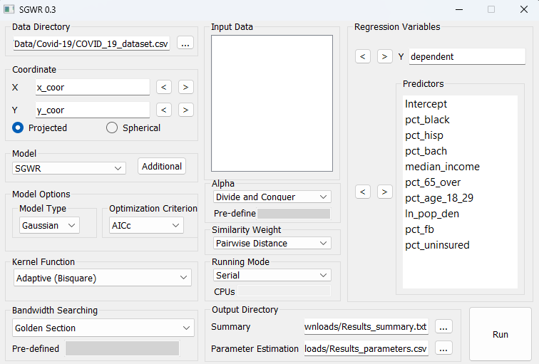
Further implementation details, including a video demonstration, are available on the Penn State GIScience website.
The SGWR Python package provides both sequential and MPI-parallel implementations for the SGWR model; however, for the M-SGWR model, it contains only the serial mode in the current version. To install the package, use pip install sgwr, and then follow the guidance below to run the models. Before fitting the model, users should prepare point-based spatial data and import the required Python libraries. If the original dataset is polygon-based, point coordinates such as polygon centroids should first be generated because SGWR requires coordinates for distance calculations. In the sequential implementation, the principal inputs are the coordinate pairs (u, v), dependent variable y, predictor matrix X, and the predictor data used to construct the attribute-similarity weight matrix.
Sequential fitting, kernel choices, model diagnostics, MPI execution, and command-line options.
Click Here for GuidanceSerial multiscale fitting with AICc or cross-validation optimization and model-result extraction.
Click Here for GuidanceLessani, M. N., & Li, Z. (2024). SGWR: Similarity and geographically weighted regression. International Journal of Geographical Information Science, 1–24. Access
Lessani, M. N., Li, Z., Yu, M., Greatrex, H., & Shen, C. Multiscale Similarity and Geographically Weighted Regression (M-SGWR). Access
Lessani, M. N., & Li, Z. (2025). Enhancing the computational efficiency of the SGWR model and introducing its software implementation. Annals of GIS, 1–16. Access